Income is generated through the production process and that income will be spent to purchase goods and services.

The components of aggregate expenditure are as follows

• Private consumption
• Government consumption expenditure
• Investment expenditure
• Net export

The consumption expenditure depends on the disposable income. C = f (Yd)

Private consumption expenditure comprises

• Buying durable consumer goods
• Buying non durable consumer goods
• Buying services

The expenditure on capital goods is, investment expenditure .Example: Machinery, tools, housing and etc.

Government expenditure spent to purchase goods and services from private sector to provide various economic activities.

Example:

• Provide public goods
• Provide merit goods
• National security
• Government administrative cost

The difference between export revenue and import expenditure is net exports
This net export can be either negative or positive.

The determinants of private consumption can be shown as follows.

• Disposable income
• The wealth of households
• Levy of taxes by the government
• Loans of households

• The determinants of investment expenditure are; as follows Demand for goods produced through new investments.
• Changes of interest rates and corporate taxes.Business expectations

The factors of determining the government consumptions expenditure are as follows

• Usage of public goods
• The expenditure on welfare goods
• The expenditure on public administration

Aggregate income (Y) and aggregate expenditure (E) are equal in macroeconomic equilibrium.

This can be illustrated through two approaches.

• Withdrawers and injection approach
• Income and expenditure approach
• Income and expenditure approach illustrates the equilibrium in a simple economy as,
  Aggregate income= Aggregate expenditure  Y = E
• In a simple economy the determinants of aggregate expenditure (E) are Private consumption expenditure and investment expenditure
• It can be illustrated with the following equation E= C+I

Aggregate income is utilized for consumption expenditure and savings in a simple economy
It can be illustrated with the following equation. Y = C+S

With withdrawers and injections approach, the equilibrium in a simple economy can be
illustrated as follows
Y = C+S
E = C+I
Y = E
C+S = C+I
S = I
Savings are withdrawers (W) and investments as the injections (J). Therefore with- drawals and injections are equal in the equilibrium.
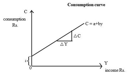
The consumption function can be illustrated as follows.

C = a+byd C = Consumption
a = autonomous consumption
b = Marginal propensity to consume
y = Disposable income
Autonomous consumption is determinants independent of current income.

Marginal propensity to consume shows the fraction of change income which is
consumed.
It can be calculated as follows

MPC = ΔC/ΔY
b = Marginal propensity to consume (MPC)
Δc = Change in consumption
Δy = Change in income

The consumption function can be illustrated with a graph.

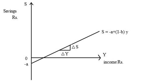
Saving function also can be illustrated as
S = -a + (1-b) yd
S = Savings
a = autonomous savings
(1-b) = Marginal propensity to save (MPS)
Marginal propensity to save shows that a fraction of change in income which is saved. It can be calculated as

MPS = ΔS/ΔY
ΔS = Change in savings
ΔY = Change in income
MPS = Marginal propensity to save
Saving function also can be illustrated graphically.

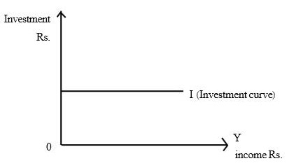
Assuming that though the income is changed, the investment is constant in a simple
economy According it, the investment can be shown as

Equilibrium in a simple economy can be computed with,

• a schedule
• graphical presentation
• Equations

Equilibrium can be calculated with a schedule in a simple economy

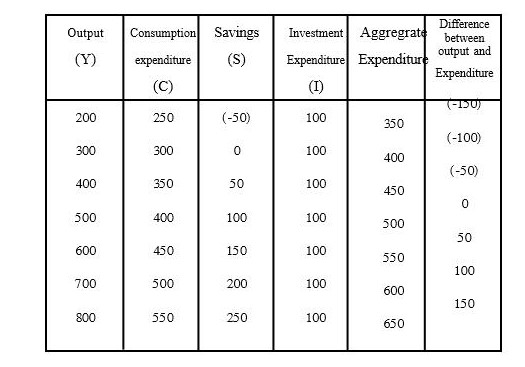
The equilibrium of a simple economy can be computed graphically

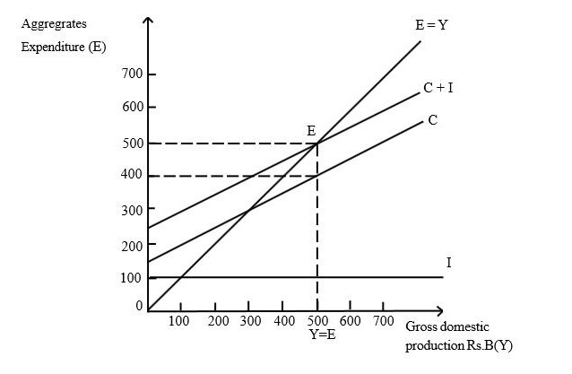
According to the diagram, national Income is illustrated with the point E.
The equilibrium in a simple economy can be calculated with the graph and equations
also.

Change in equilibrium in a simple economy depends on the following components.

• Change in consumption function.
• Change in investment.

Change in consumption function depends on two factors.

• Change in autonomous consumption
• Change in Marginal Propensity to consume (M.P.C)

Change in consumption function can be illustrated with the change in autonomous consumption.

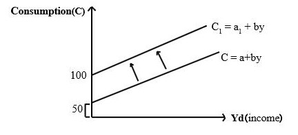
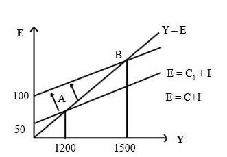
According to the above diagram, the consumption function has changed due to the change in autonomous consumption.
The aggregate expenditure curve has also shifted due to the change in consumption curve.
The equilibrium output level has also changed.
The equilibrium level can be changed with the change in Marginal Propensity t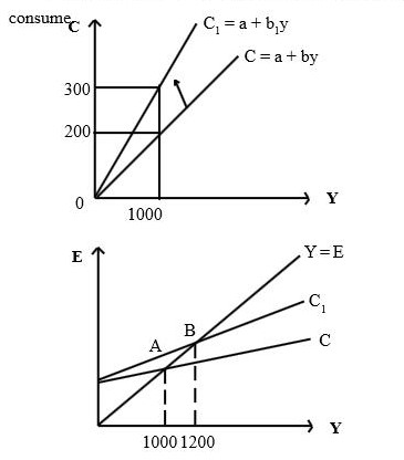

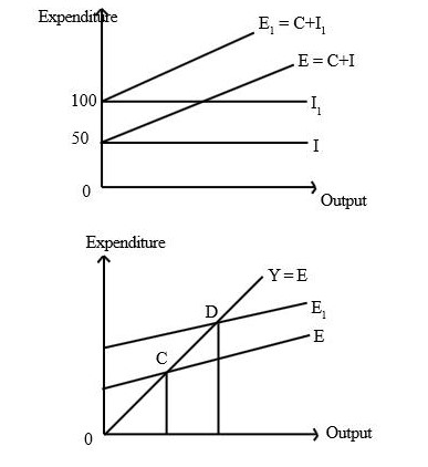
• The slope of the consumption curve is changed because of change in marginal propensity to consume.
• Slope of Aggregate expenditure is also changed with the slope of consumption curve.
• The equilibrium level has also changed. In a simple economy, the equilibrium
  level has also changed due to change in investment.

Investment curve is changed due to change in investment.
When investment curve is changed, the expenditure curve also will be changed.
Therefore the equilibrium level of output also will be changed.

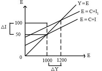
Because of the change in autonomous expenditure, the influence to change the output is
explained as the multiplier effect. (K)
The change in the autonomous expenditure of a simple economy, that is the
autonomous consumption and autonomous investment influence the multiplier effect.
Multiplier in a simple economy can be computed as follows.
Multiplier in a simple economy = K

K=1/(1-b)

b= Marginal Propensity to consume

• This can be explained with a simple example. change in autonomous expenditure causes to change the output
This can be illustrated with the multiplier.

Y =  (1/(1-b) )X ΔI

ΔY = Change in income
ΔI = Change in autonomous investment

• Change in output is computed with a multiplier when autonomous expenditure is changed.
  This is explained with the following example.
  Assuming Marginal Propensity to consume is 0.75 when investment (I) is increased
  from 50 to 100.
  Change in output is ,

ΔY =  1/(1-b) X I

ΔY = (1/ (1-0.75) )X (100-50)

ΔY = 4 x 50

ΔY =200

This can be illustrated with the following diagram

Multiplier effect can be also explained with a statistical table example.

Equillibrium level of output depends on a level of full employment or  outer.