The main variables which decide the economic activities are known as macro economic variables.

Macro economic variables can be shown as follows

• National output
• Employment
• Price level
• Balance of payment
• Foreign exchange rate.

 

• When the activities of the main economic variables change, the aggregate production
  of the economy also changes.
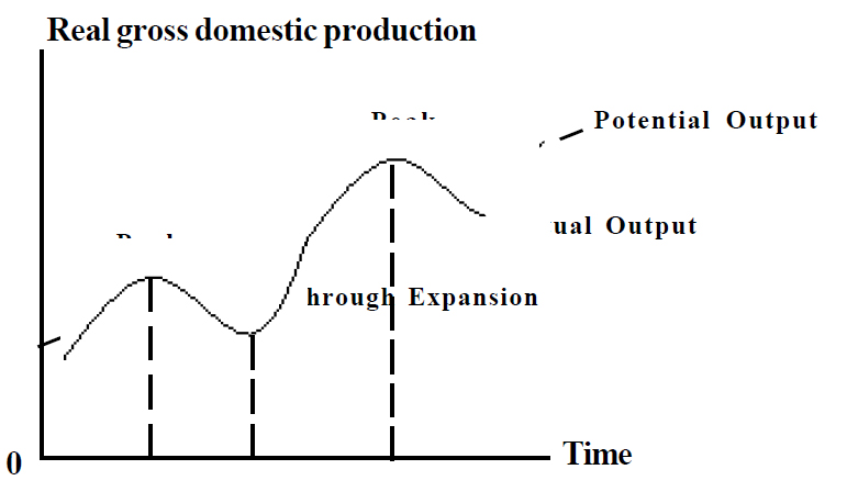
• Business cycles are explained as the cyclical behaviour of real gross domestic
  production which changes with time.
• Business cycles can be used to understand the relationship of short term and long
  term behaviour of a macro economy.

Can understand the four periods of a business cycles.

• Recession
• Trough
• Expansion
• Peak

This can be illustrated with a graph.

• The point where the actual output is at its minimum, is trough; and maximum point of
  the actual output is peak.
• The period from trough to peak , is the period in which the actual production is expanded.
• The period from peak to trough is the periods in which the actual production is
  constructed; and this the recession.
• Time periods of expansion are longer than recession .
• Time from one peak to another peak is the length of a business cycle and these lengths
  vary in a business cycle and lengths vary with each other.
• The long term trend of a business cycle can be explained as either economic growth or
  economic decline.

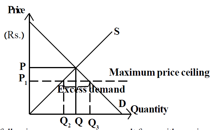
Government intervenes, when market equilibrium which is decided by market forces of demand and supply, are unfavourable to society, to introduce control price, which is explained as price control policy.

 

• Implementing a maximum price legally is termed maximum price ceiling.
• If the maximum price is to be effective it should be lower than equilibrium price.
• Implementing a maximum price ceiling can be illustrated using a following
  diagram.

The following consequences can result from with maximum price policy.

 

• Shortage of goods.
• Non price rationing
• Creation of a black market price
• Creation of a economic inefficiencies

 

The following diagram illustrates a how black market occurs with maximum price policy.

 

 

C+E = Loss of economic surplus
P2 = Black market price

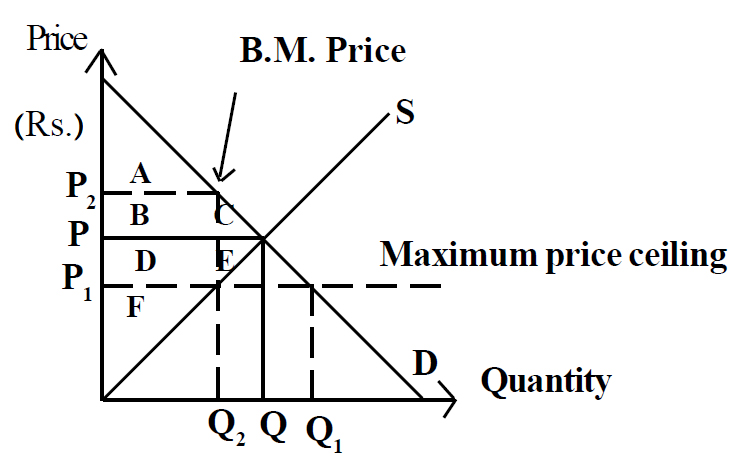
The following diagram illustrates how economic inefficiencies occur with
maximum price policy

 

Economic surplus before price ceiling A+B+C+D+E+F.

After price ceiling policy consumer surplus is only A. and producers surplus is only F.

After implementing maximum price ceiling policy economic, surplus of C+E is a loss to society.
If consumer does not have to pay an extra amount to purchase scarce goods except A,B and D will be added to consumer surplus.

 

The following methods can be shown to clarify maximum price.

• Rationing
• Imports
• Incentives for the production.

Non price rationing measures can be illustrated as follows

• Queues
• Use of ration cards
• Rationing with bribes
• Distribution is connected with other goods.

 

•  Goods can be imported as a solution for the shortage created in market as the result of a
  price control policy.
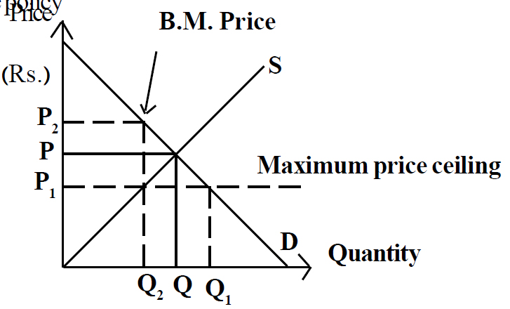
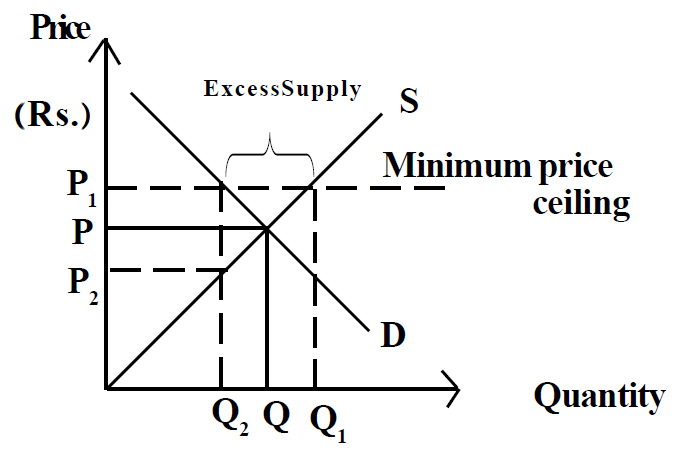
•  Minimum price is explained as the price which is implemented higher than equilibrium
  price to give a better price for producer and factor owners.
•  If minimum price is implemented lower than equilibrium price, the objectives of minimum
  price policy cannot be obtained.

Minimum price implementation can be illustrated with the following diagram.

 

• The following consequences can occur in the market with minimum price policy.
•  Excess supply or surplus of supply.
•  Unemployment can occur when minimum price is implemented in the labour market.
•  Excess investment situation can occur.
•  Goods can be supplied to consumers at discounted rates by keeping minimum price as
  nominal price.

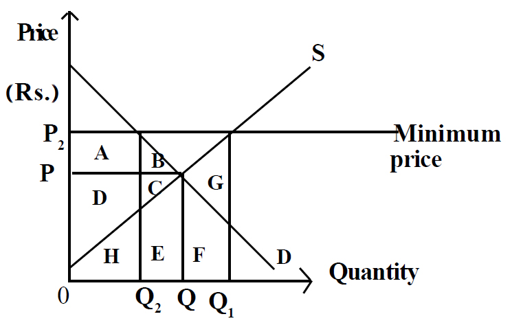
 Welfare effects of minimum price policy can be illustrated with the following diagram

When implementing minimum price consumer surplus, producer surplus will be
changed.

 

The following steps can be taken to clarify minimum price.

• Hoarding excess supply
• By products
• Promoting demand.
• Exports

Government can implement a price support policy with minimum price to give a higher income to producers

• after implementing minimum price policy, it market supply is limited to Q
  2,the welfare loss to society will be B and C
• If the producer decides to expand the market supply up to Q1 after implementing minimum price policy the welfare loss the society cannot be assured.
• If the producer decides to expand market supply to Q1 after implementing minimum price policy and if the government purchases the excess supply the welfare loss to society will be B+C+E+F+G

Subsidies can be implemented on the producer in two ways

• Unit or specific subsidy
• Ad Valorem subsidy

 

Providing a specific amount on one unit of production is explained as a unit
subsidy.

Taxes can be implemented on producer in two ways

 

• Specific tax or unit tax.
• Advalorem tax
• Unit tax is a specific rate on a production unit which is sold.

 

Taxes can be implemented on the producer in two ways

Tax incidence is divided according to the demand and supply elasticity can be explained graphically.

 

• The consumer bears the total tax incidence in perfect inelastic demand.
• The producer bears the total tax incidence in perfect elastic demand.
• Tax burden is divided equally between the consumer and producer in a unitary
  elastic demand.

 

• Inelastic demand more tax burden should be borne by the consumer, and the producer bears less tax burden.
• Inelastic demand more tax burden should be borne by the producer, and the consumer bears less tax burden.

 

• The producer bears total tax incidence in perfect inelastic supply.
• The consumer bears total tax incidence in perfect elastic supply.
• Tax incidence is divided equally between consumer and producer in unity elastic
  demand.

 

• The producer has to bear more tax incidence in inelastic supply.
• The consumer has to bear more tax incidence in elastic supply.

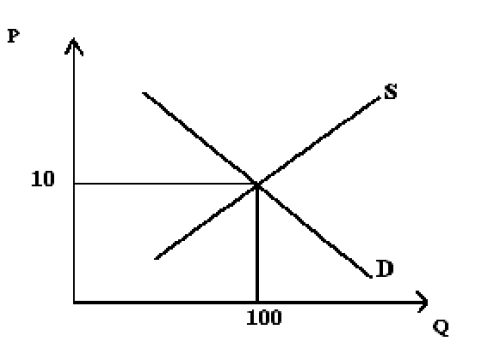
Price is determined by demand and supply in a Perfect Competitive industry.
It can be illustrated by the following diagram.

• Price which is determined as above, cannot be changed by one firm, therefore activities of a firm will be inactive.
• A firm can produce any amount of at the market determined price.
• Therefore a production in a Perfect Competitive firm is a price taker.
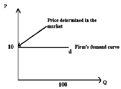
• A firm can supply any amount of goods at the prevailing price.
• Any amount of goods can be demanded at that price.
• The demand curve of a Perfect Competitive firm is perfectly elastic.

This can be illustrated with following diagram.

The production in short term is governed by technology and capacity of the firm.
Output and cost is divided on these components.
To obtain maximum loans in a short run, two important decisions should be taken. They are normally,

• Whether production should continue or close down?
• If production is to be continued, what is the amount of production?

 

• When deciding on output level according to maximization of profits, firms have to follows two alternative of profits, the firm has to follow two alternatives namely,
• Deciding on output level of maximum economic profits based on revenue and cost.
• Deciding on output level of maximum economic profits based on marginal revenue and total cost
• The total amount of money which a firm earns by selling its output to the market is termed as Total revenue.
• Total revenue can be calculated by multiplying quantity and price of good.
  TR = Q x P
  Total Revenue = Output x Price.

 

• Average revenue can be calculated by dividing Total revenue with quantity of goods

          AR = TR / Q
          Average Revenue = Total Revenue/ Output

 

• Change in total income, when producing one more extra unit is termed as marginal revenue,
• Change in total revenue should be divided by change in output to reach marginal revenue.

          Marginal Revenue = Change in Total Revenue / Change in output

          MR = ΔQ / Δ TR

 

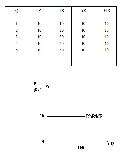
• Determined price can be seen in a perfect competitive firms, therefore price of good, average revenue marginal revenue are equal to each other.
• Then P=AR=MR Concept is fulfilled.
• To illustrate relationship between Total Revenue average revenue and Marginal
  Revenue,

Following schedule and graph can be constructed.

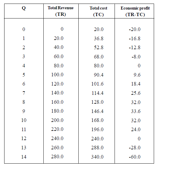
• Economic profits can be gained by deducting total cost from total revenue.
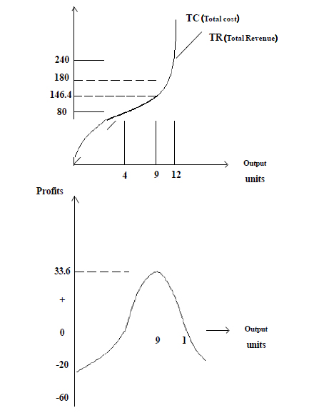
• Relationship between total cost, Total revenue and economic profits can be illustrated by a schedule and a graph.

• According to the above schedule and the diagram the following factors can be concluded.
• Revenue curve will commence through the origin and slope upwards as the revenue is increased with inverse in output.
• Cost curve slopes upwards, as cost is increased with increase in output..
• Economic profit will be zero when the total cost and revenue curve intercept each other.
• If the total cost curve is higher than the revenue curve, economic losses can occur or zero economic profits.
• If the total revenue curve is higher than the total cost curve, economic profit occur.
• Economic profits will be maximize at mid point where the highest difference between the total cost curve and the total revenue curve.
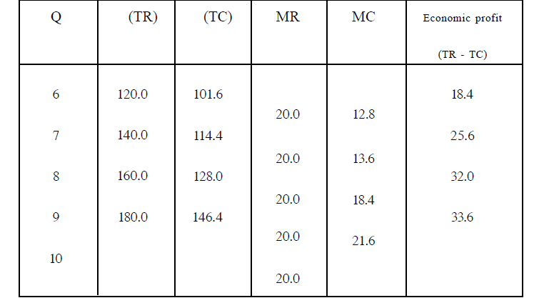
• Marginal costs (MC) and marginal revenue (MR) analysis also can be used to illustrates
  profit maximization.
• If marginal cost is less than marginal revenue(MR>MC) it means the firms will make
  extra profits by selling more units.
• If marginal revenue is less than marginal cost (MC>MR) firms will take losses by
  producing extra units.
• To maximize their profits, firms should produce where marginal revenue and marginal
  cost are equal.(MR=MC).
• According to marginal analysis, the output level of profit maximization should be according
  to the condition of MR=MC.
• Maximization of profit under marginal analysis, can be illustrated using the following
  schedule.

• The following factors can be gained from the above schedule.
• Economic profits will remain between 8th and 9th units of production.
• Firms leave to reduce profits between 9th and 10th units of production.
• At the 9th units of production there is no increase or decrease in profits. Profits are
  maximized.

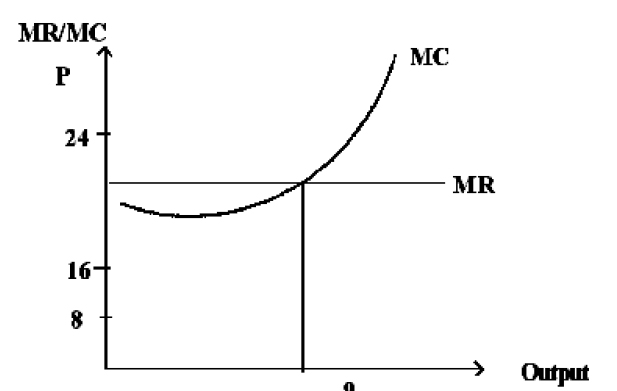
Profit maximization of a perfectly competitive firm can be illustrated through the following
diagram.

According to the above graph,

• If the output is less than 9 units profits can be increased by increasing the output.
• At the 9th unit economic profits are maximized.
• If the output is more than 9 units economic profits will decrease.
• Economic profits will remain between 8th and 9th units of production.

Short run behaviour of a perfectly competitive firm, can be explained through three alternative situations. Such as,

• Producing earnings with economic profits
• Producing earnings with zero economic profits
• Producing earnings with economic losses
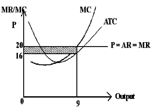
• When economic profits are earning, the selling price of a unit is more than the average total cost (ATC/AC).

This can be illustrated through the following graph.

• According to the above graph, profits are maximized at the 9th unit, the total economic profits are illustrated by the schedule area.
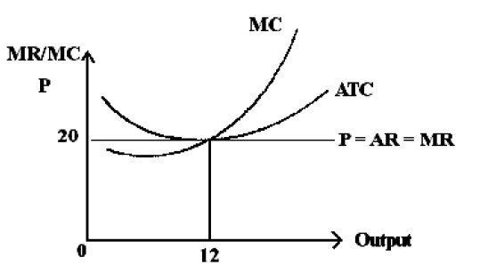
• When economic profits are zero, the selling price of a unit equals average revenue.
• This is illustrated by the following graph.

 

• Under this condition, firm will remain in the industry, because they get an income which is
  equal to average cost.
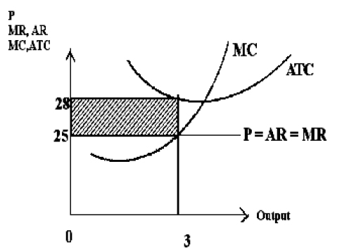
• If the selling price of the product is less than the average cost, that is with economic losses
  even a firm will produce in the short run process.
• If the losses by closing down the firm is less than that while producing , the firm will remain
  in the industry.
• This situation can be illustrated through the following graph.

• The schedule area illustrates the total losses of a firm which is producing with losses of a firm which is producing with losses in the short run.
• Perfect competition is a hypothetical market.
• A production firm can avoid variable cost in the short run but not the fixed cost.
• If the firm cannot cover up the total cost with its revenue production will be
  discount need.
• If there price is less than the average variable cost, losses will increase with
  grater production.

 
 

 

Market equilibrium is decided on demand and supply forces.

Market equilibrium can be explained in three ways

• By demand and supply schedules.
• By graphs.
• By equations.

Concepts which are related to market equilibrium can be shown as follows

• Excess demand.
• Excess supply
• Excess demand price
• Excess supply price
• Consumer’s surplus
• Producer’s surplus

 

• Demand exceeds supply at a given price is termed excess demand.
• Supply exceeds demand at a given price is termed excess supply.
• Excess supply price occurs below the market equilibrium price, .
• Excess supply price occurs above the market equilibrium price .
• The difference between the price which the consumers are willing to pay for equilibrium quantity and actual price which they pay is explained as consumer’s surplus.

 

• The difference between the producers minimum expected price and the actual price which they get is termed, producer’s surplus.

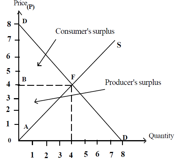
Consumer’s surplus and producer’s surplus can be illustrated with following graphs.

 

 

According to the above graph the surface area of BDF shows consumer’s surplus.
The consumer’s surplus can be computed using the following formula.

Consumer’s surplus =  {  (Maximum price-equilibrium price x quilibrium Quantity) / 2 }

 

 

According to the above graph the surface area of ADF shows producer’s surplus.
Producers surplus can be computed using following formula

Producer’s surplus = { (Equilibrium price – minimum price) quilibrium Quantity / 2 }

 

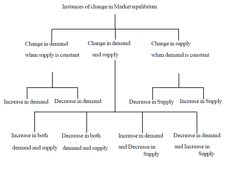
Market equilibrium can be changed with the changes of either demand or supply of the market or changes of supply of the market or changes of both demand and supply

This can be illustrated through the following chart Instances of changes in market equilibrium

 

Changes of equilibrium with market forces can be explained through graphical
presentation
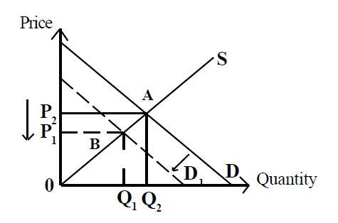
Examples of changes in equilibrium with decrease in demand while supply is constant

E- equilibrium before change in demand.
E1 – equilibrium after change in demand

 

Calculations of elasticity of supply on a point of a supply curve is explained as point of elasticity.

 

The point elasticity of supply can be illustrated by the following formula / equations

E =  { (ΔQS/ΔP) X (P/QS)
Axe elasticity of supply is explained as elasticity between two points of a supply curve in given period of time.
Arc elasticity of supply is calculated using the following formula.

 { (ΔQS/ΔP) X (P1+ P2 /QS1 +QS2) }

Five range of price elasticity of supply can be illustrated as follows.

•  Perfect inelastic supply
• Inelastic supply
• Unitary elastic supply
• Elastic supply
• Perfect elastic supply

 

• The supply curve with a positive intercept illustrates elastic supply.
• The supply curve with a negative intercept illustrates inelastic supply
• The supply curve passing through the origin illustrates unitary elasticity of supply.

In addition to the above situations there is perfect inelastic supply and perfect
elastic supply also.
If the supply curve is parallel to the vertical axis or the price axis price elasticity of supply is perfectly inelastic, the coefficient of elasticity of supply is zero(0).
If the supply curve is parallel to the horizontal axis or quantity axis , then the price elasticity is perfectly elastic or infinity.
Quantity supply is changed variously to a change in price because of different factors are effective.

The following are determinants of price elasticity of supply.

• Mobility of factors of production.
• Time period to supply goods
• Ability to keep stocks and production capacity
• Nature of good.

When implementing economic policies supply elasticity is very important.
Change in price to a change in the nature of a good is decided according to supply
elasticity.
Supply elasticity affects to divide tax incidence between consumer and producer when implementing taxes.
If price elasticity of supply is more elastic more benefits of a subsidy are enjoyed by the consumer
When supply of factors get perfectly elastic the total factor earnings will consist of transfer earnings.
When supply of factors get perfectly inelastic the total factor earnings will consist of economic rent.
When supply of factors get unitary elastic the total factor earnings will consist of both transfer earnings and economic rent equally.
Transfer earning and economic rent can be shown by the digams below.

• Market and industry are concepts with similar meanings.
• The sum of all firms which produce homogeneous goods is termed an industry.
• Goods and services produced by firms are sold in various market situations.
• These market situations can be termed market structures.

The following criteria can be used to classify a market structure.

Number of firms in the market.

• Nature of goods and services produced.
• Entry to and exit from market.
• Nature of competition among firms.

According to the changes of market features the nature of market structure varies / differs
Four market structures can be classified based on the above criteria.

• Perfect competition
• Monopoly
• Monopolistic competition
• Oligopoly

Market situations with ease of entry, a large number of firms which produce homogeneous products, is termed, Perfect competition

Perfect competition market has the following characteristics.

 

• Products are homogeneous
• A large number of buyers and sellers are present in the market
• Ease of entry to the market
• Perfect information can be taken about a market.

Close characteristics of Perfect competition could be seen in the agriculture, fishing, industry and mining industry

Market situations with one industry and one firm and barriers to entry is termed monopoly.

A Monopolistic market has the following characteristics.

• Only one firm is involved in production
• Specialty in production
• Barriers to entry to the industry
• Imperfect information on the market

Because one firm is in a monopolistic market, it can influence market price
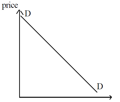
Demand curve of monopoly is a downward sloping curve.
It can be illustrated as follows.

Supplier of monopolistic firms acts as a price maker.
Examples of a monopolistic market are, water supply, electricity, railway
etc.

The following factors determine entry to the monopolistic market.

• Ownership of basic inputs -> To avoid entry of other firms to produce the good.
• Government legislator obstructions -> Goods should be produced under government licences..
• Returns to scale -> Producing goods by institutions which are involved in the market ( Natural Monopoly).

Both characteristics of Perfect competition and Monopoly can be seen in a market situation which is called Monopolistic competition

The following characteristics can be illustrated in a Monopolistic competition market

• A large number of sellers.
• Differentiated goods.
• Ease of entry.
• Most exceptional characteristics of Monopolistic competition is differentiation of goods.
• Goods differentiation means, that every firm will differentiate his good with
  other supplies and provide it to the market.
• Because of differentiation of goods, one good of a firm is not a perfect
  substitute to another good of another firm
  Examples – different soaps, Tooth paste and Shoes

Because of differentiation of goods, production firms have to compete with each other, and this ability will strengthen them with the following factors.

• Quality of these good
• Price of good
• Marketing

 

• The demand curve of a monopolistic competitive market slopesdownwards.
• Oligopoly is defined by a limited number of firms in the market.

 

The following characteristics can be seen in Oligopoly

• These is a artificial or natural barriers to limit new firms entering the
  industry.
• There is a small number of firms competing in industry.
• Market imperious. (Imperious attitude in market)

The following are the barriers to limit new firms entering the industry

• Returns to scale.
• Goodwill.

 

• Because of a small number of firms in market the portion of market for each firm is relatively high.
• Therefore firms in the market are interdependent.
  Examples of Oligopolistic industries are newspapers, broadcasting
  services, soap, soft drinks commercial bank, Gas etc.

• Qunatity supply is changed with the change in price of good concerned when all other factors which determine demand remain constant.
•  If all other factors which determine supply, are constant , increase in price causes to the quantity supply to decreases, then a point on the supply curve movesdownwards along supply curve.
•  When all other factors which determine supply, the increase in price causes increase in quantity supply and a point on the supply curve moves upwords along the supply curve.

Decrease in supply or increase in supply happens if all other factors change while the
price of the good concerned is constant. Increase in supply causes the supply curve to shift to the right.

The following reasons causes the supply curve to shift to the right.

• Decrease in price of related good
•  Decrease in price of production inputs
• Improvements of technology
• Expecting a price increase of a good concerned in the future.
• Increase in the number of producers in a market.
•  Providing subsidies to producer by the government.
• The supply curve will shift to the left when the supply decreases.

The following reasons cause the supply curve to shift to the left.

• Increase in the price of related good.
• Increase in the price of production inputs
• Deterioration of technology
• Expecting a price decrease of good concerned in the future.
•  Decrease in the number of producers in the market.
• Imposition of taxes on goods and services by the government.

Components of the short run costs of production can be stated as below

• Total fixed cost
• Total variable cost
• Total costs
• Marginal cost
• Average cost
• Average fixed cost
• Average variable cost

 

• Fixed costs are expenditure on fixed factors such as Machinery, plants and management
• Fixed costs exist even if zero output is produced
• Total variable costs are expenditure on variable factors such as raw materials and labour
  used in the production
• Total cost is all expenditure incurred in the production of a commodity
• Total variable cost is zero when the output is zero. As output is increased total variable
  costs increase first less rapidly and then more rapidly. The reason is the law of diminishing
  returns.
• Total cost consists of fixed costs and variable costs.

 

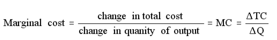
• Marginal cost is the change in total costs as one more unit of output is produced. It is calculated as follows

 

• Average total cost (ATC) is the total cost per unit of output
• Average total cost is calculated as follows
• Various forms of short run costs of production can be calculated
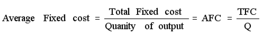
• Average total fixed cost (AFC) is the total fixed cost per unit of output It is calculated as follows

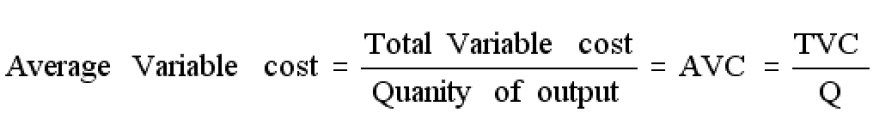
• Average variable cost (AVC) is the total variable cost per unit of output It is calculated as follows

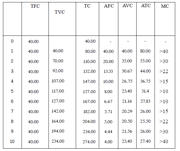
• The above cost components can be presented in a schedule as below

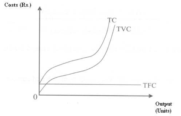
• Total cost, total fixed cost and total variable cost given in the schedule can be illustrated graphically as below

• Marginal cost, average cost, average fixed cost and average variable cost given in the schedule can be illustrated graphically as below